Installing the GUI#
Install the graphical interface to inspect and retrieve a FROG trace without writing Python. uv supplies Python and creates an isolated environment for croak. You will use a terminal for installation and launching; subsequent analysis takes place in the GUI’s window.
Before you start#
You need an internet connection for installation. On macOS, open Terminal; on Windows, open PowerShell; on Linux, open your usual terminal. Copy the commands for your platform below. The installation reference covers platform requirements and optional features.
1. Install uv#
macOS / Linux:
curl -LsSf https://astral.sh/uv/install.sh | sh
Windows (PowerShell):
powershell -ExecutionPolicy ByPass -c "irm https://astral.sh/uv/install.ps1 | iex"
Or brew install uv on macOS. See the
uv install docs for
other options.
2. Install croak#
uv tool install --python 3.14 "croak[gui]"
uv downloads the right Python (3.14) if you do not have it, creates an
isolated environment, installs croak with the Qt interface from PyPI, and puts
the croak-gui command on your PATH. No system Python is touched.
On Linux, install the Qt system libraries if they are missing.
3. Run it#
croak-gui
If the shell cannot find croak-gui, run uv tool update-shell and open a new
terminal. See uv’s tool guide for PATH
configuration. If the window fails to appear on Windows, run
uvx --python 3.14 --from "croak[gui]" python -m croak.gui to display diagnostic
output in the terminal.
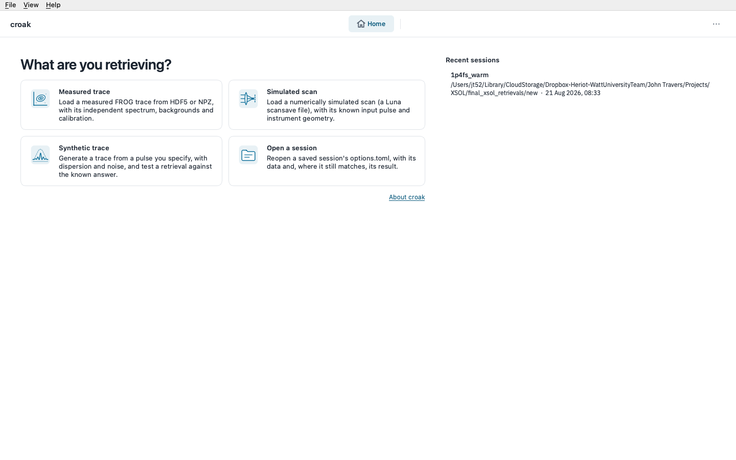
The window opens maximised and is laid out for displays of 1366×768 and up; un-maximised, it returns to the size you last left it. It opens on Home:
4. Use it#
Pick a tile on Home — Measured trace (an HDF5 or .npz file, with an
optional independent spectrum from HDF5, .npz or CSV and calibration curves
from CSV), Simulated scan or Synthetic trace (a pulse you specify, to try
croak without data). The session then runs through five stages, shown as
buttons in the top bar:
Data — load (or generate) the trace;
Check — compare its frequency marginal with the independent spectrum;
Prepare — filtering, background removal, windowing and regridding;
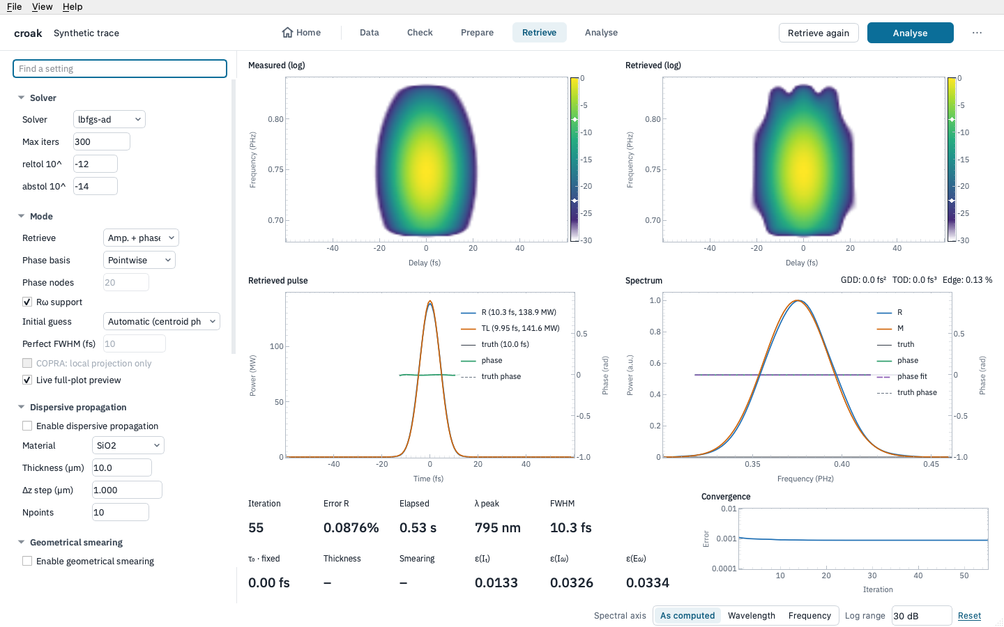
Retrieve — choose a solver and run it, with a live preview;
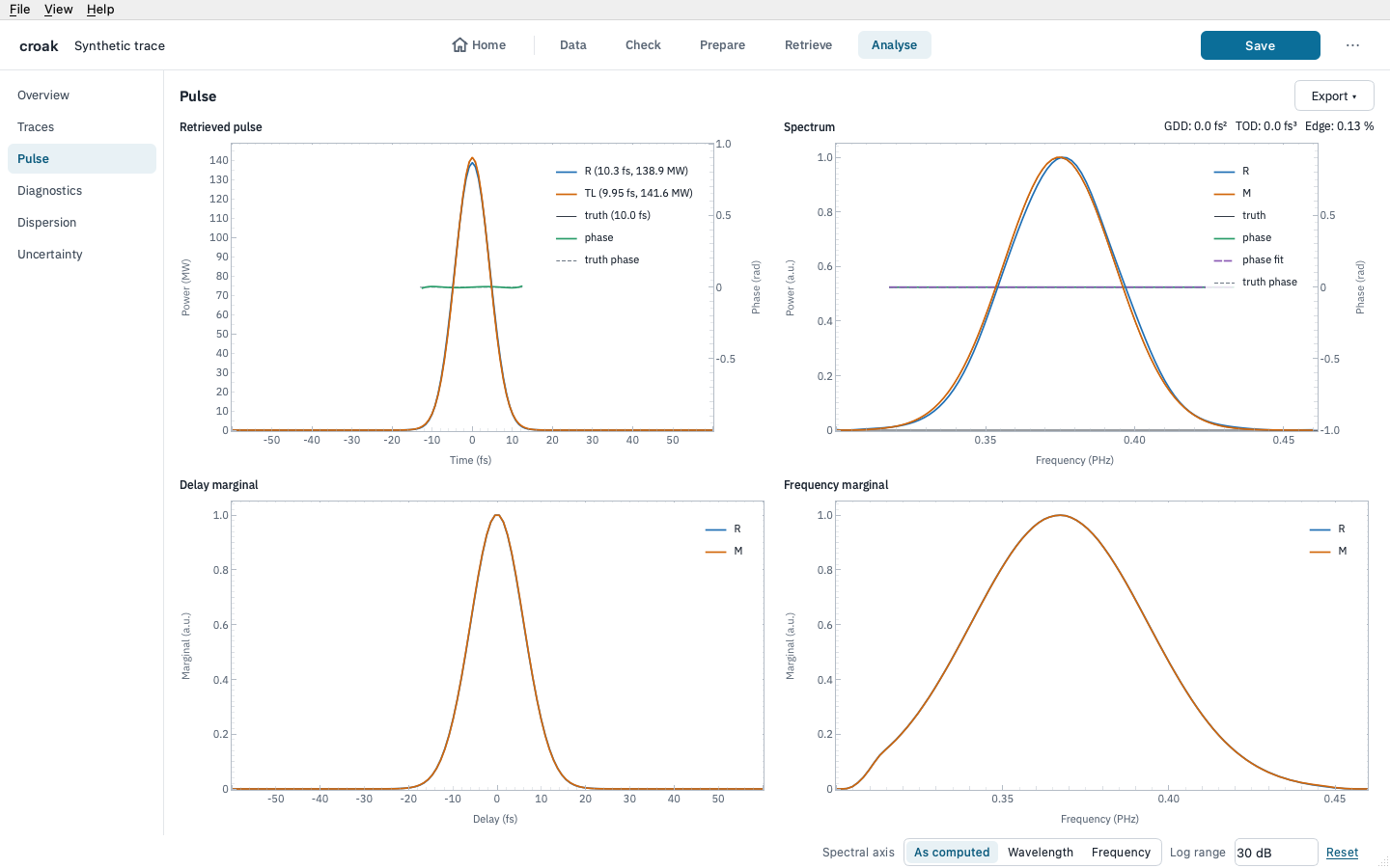
Analyse — the retrieval’s pages of panels, then Dispersion (tuning with materials and chirped mirrors) and Uncertainty (error bars on the retrieved duration).
The button at the right of the top bar does the next thing — Continue, Retrieve, Save — and a stage you cannot open yet is greyed out, with the reason in its tooltip; Home at the start of the row goes back to Home. Settings are in a narrow column on the left of each page and the plots fill the rest; hover over a control for help with that setting, and over a plot to read its values. Scroll to zoom, drag to pan, and double-click to return to the starting view. Right-click a plot, or press Ctrl+E (⌘E) for the whole page, to save it as a figure for publication: a vector PDF or SVG drawn by matplotlib. At the foot of the window, Spectral axis draws every spectral plot against wavelength or frequency, and Log range sets how far down every logarithmic map reaches; drag a map’s colour bar to adjust that map alone.
The GUI guide documents each stage in detail. Save
session… in the ⋯ menu writes the retrieval, a TOML file that records every
setting and an overview PDF into a folder (with the dispersed pulse and the
uncertainty figure, when Analyse holds them), and the session then appears under
Recent sessions on Home. A saved session can be re-run later — including
headlessly with croak replay options.toml — or exported as a standalone Python
script with croak script options.toml (the croak command is installed
alongside croak-gui).
Updating#
uv tool upgrade croak
If you would rather run from a checkout of the source — for example to try the
bundled examples too — clone the repository and use
uv sync --extra gui then uv run croak-gui from the croak directory; see
Installation.